Master Class: How Wireless Sensor Networks Adapt to Earth’s Five Most Extreme Environments

Modern Wireless Sensor Networks and Edge IoT Systems

Introduction: The Core IoT Engineering Trade-Off

A Wireless Sensor Network (WSN) is a system of spatially distributed, autonomous devices equipped with sensors, processing elements, and transceivers. These devices collaboratively monitor physical or environmental conditions and route telemetry across network topologies to a centralized infrastructure. In controlled laboratory settings or consumer smart homes, deploying IoT hardware is straightforward: power outlets are readily accessible, ambient temperatures remain stable, and Wi-Fi or cellular coverage is virtually guaranteed.

However, when sensor networks are pulled out of clean indoor labs and deployed into real-world operational domains, physical wiring becomes economically unfeasible, structurally impossible, or hazardous. In these unmanaged spaces, every design choice is forced to confront the Universal Engineering Dilemma—an ongoing balance across three antagonistic requirements:

Transduction Fidelity: Capturing weak, noise-sensitive physical signals (such as micro-volt biopotentials, structural vibrations, or subtle gas concentrations) with absolute mathematical accuracy.
Communication Range and Reliability: Guaranteeing data delivery across lossy, dynamic, or radio-opaque media without dropping critical frames.
Energy Autonomy: Sustaining continuous operation over multi-year or multi-decade lifespans from finite batteries or scavenged ambient energy.

Failure in any single dimension collapses the system’s operational utility. A node that consumes its entire battery in a week, loses radio lock inside a concrete pier, or outputs corrupted sensor readings due to electromagnetic interference is useless in the field.

In extreme IoT, environment drives architecture; network design must be derived from the governing equations of the physical domain.

To build resilient systems, engineers must stop forcing standard commercial wireless protocols into specialized settings and instead let the physics of the environment dictate every layer of the hardware and software stack. This foundational rule becomes immediately obvious when moving from general IoT concepts to the physical challenges of monitoring massive civil infrastructure.

Structural Health Monitoring (SHM): The Precision & Timing Challenge

Civil infrastructure assets—such as suspension bridges, concrete dams, mountain tunnels, and high-rise buildings—are subject to continuous physical degradation from traffic loading, material fatigue, seismic events, and ground settling. Structural Health Monitoring (SHM) networks are deployed to detect microscopic structural fatigue, displacement, and modal vibration shifts long before catastrophic structural failure occurs.

The Physical Challenge

Operating on large civil structures introduces severe physical obstacles:

Environmental Signal Masking: Natural diurnal temperature cycles induce thermal expansion and contraction across structural members. These environmental shifts produce mechanical strain signals that can mask or mimic structural degradation. Sensor processing units must continuously run baseline temperature-normalization algorithms to isolate actual mechanical damage from ambient thermal expansion.
RF Attenuation in Concrete and Steel: High-frequency radio signals struggle to penetrate steel-reinforced concrete piers, massive abutments, and metal suspension towers. Engineers must carefully align directional patch antennas and strategically place repeater nodes to maintain reliable line-of-sight communication paths.

Transducer Mechanics

Capturing structural health requires specialized transducers that convert physical deformation into measurable electrical signals:

Seismic MEMS Accelerometers: Measure ambient, wind-induced, or traffic-induced micro-vibrations with noise densities below 20,\mu\text{g}/\sqrt{\text{Hz}}. These sensors capture dynamic response parameters, such as natural frequencies, mode shapes, and damping ratios.
Vibrating Wire Strain Gauges: Feature a tensioned, high-strength steel wire clamped directly to a structural member. An electromagnetic coil plucks the wire and measures its resonant frequency (f). As structural elements undergo mechanical strain, wire tension changes according to the relationship: \Delta \epsilon \propto \Delta f^2 These sensors naturally resist electrical noise and maintain mechanical stability over multi-decade deployments.
Fiber Bragg Grating (FBG) Optical Sensors: Etched into optical fibers interfaced with wireless interrogators, FBGs reflect a narrow band of light known as the Bragg wavelength (\lambda_B), defined by: \lambda_B = 2 n_{\text{eff}} \Lambda Physical deformation shifts both the grating period (\Lambda) and the effective refractive index (n_{\text{eff}}), allowing fine-grained strain measurements without electrical spark risks.
Linear Variable Differential Transformers (LVDTs): Measure minute expansions and contractions across seismic expansion joints with sub-millimeter precision by tracking mutual inductive coupling shifts between a primary center coil and two secondary outer coils as a ferromagnetic core slides inside the assembly.
Electrolytic Tiltmeters: Measure precise angular shifts and rotational settling in bridge piers and dam abutments by monitoring electrical resistance changes across fluid-filled electrolytic cells as internal bubble movement unbalances a conductive bridge circuit.

Network & Timing Solution

Modal vibration analysis relies on calculating the relative phase shifts between spatially separated sensor nodes across a bridge or dam. If node clocks drift independently, calculated mode shapes fail, making structural diagnostics inaccurate. Consequently, standard contention-based CSMA/CA MAC protocols are completely unsuitable due to their variable queuing latencies and clock drift.

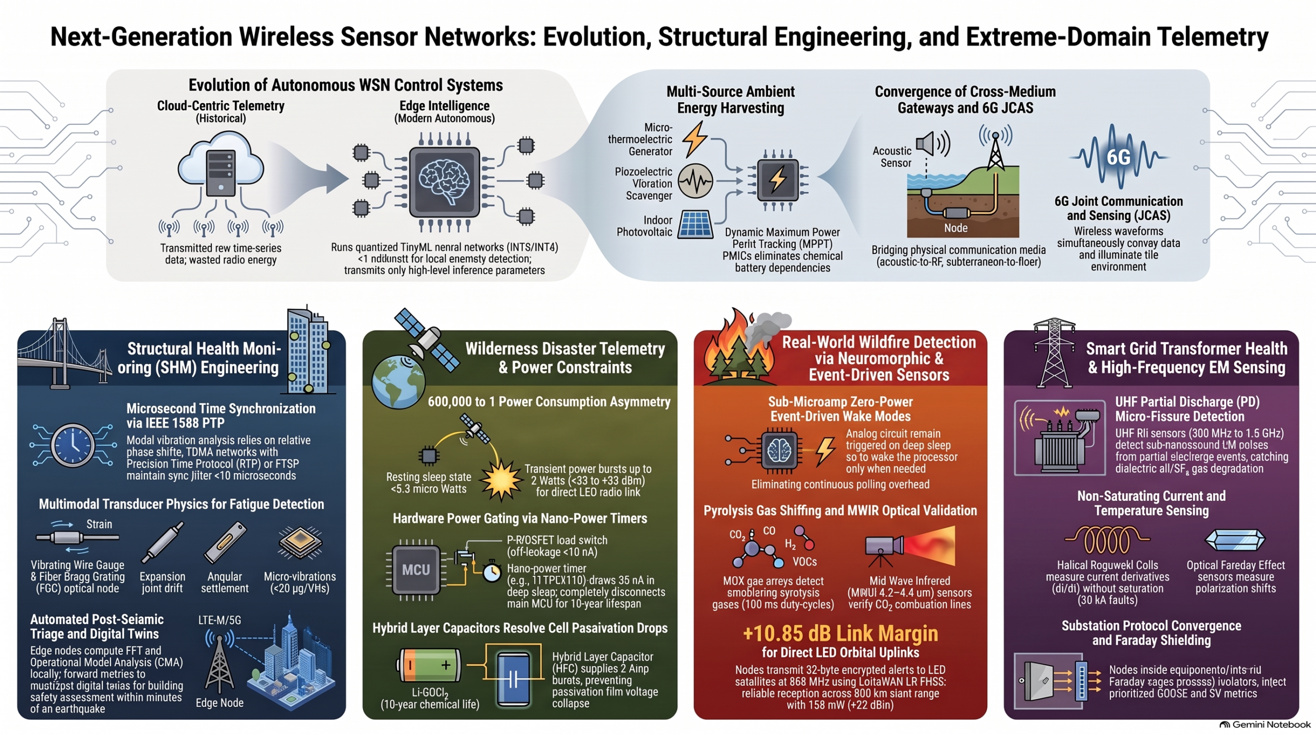
To overcome this, SHM networks implement Time-Division Multiple Access (TDMA) combined with the Precision Time Protocol (PTP / IEEE 1588) or Flooding Time Synchronization Protocol (FTSP). This architecture maintains clock synchronization jitter below 10,\mu\text{s} (sub-10 microsecond precision) across all nodes in the mesh. Microcontrollers at the edge run high-frequency sampling engines and localized Fast Fourier Transforms (FFT) to perform Operational Modal Analysis (OMA), extracting peak vibration frequencies and mode shapes locally before transmitting processed telemetry to central concentrators.

While structural monitoring demands extreme sub-millisecond clock synchronization across stationary concrete spans, an entirely different operational threat emerges when sensors are clamped directly to the high-voltage assets of electrical power grids.

Power Utilities & Smart Grids: Surviving the Electromagnetic Battleground

Modern power grids rely on real-time telemetry to manage Dynamic Line Rating (DLR), track transformer health, and detect arcing faults. However, operating directly on high-voltage (HV, EHV, and UHV) transmission assets operating between 69\text{ kV} and 765\text{ kV} (and up to 1,100\text{ kV}) places sensor nodes inside an extreme electromagnetic environment governed by fundamental electrodynamic laws.

First-Principles Framing

According to Ampère’s Law: \oint \mathbf{B} \cdot d\boldsymbol{\ell} = \mu_0 I A transmission conductor carrying a nominal current I = 1,000\text{ A} produces a magnetic flux density B \approx 4.0\text{ mT} at a radius r = 5\text{ cm}. During a symmetrical grid fault (I_{\text{fault}} \ge 20\text{–}40\text{ kA}), this magnetic flux spikes to 80\text{–}160\text{ mT} within a quarter-cycle. Concurrently, Faraday’s Law of Induction: V_{\text{sec}} = -N \frac{d\Phi}{dt} = -N A_e \frac{dB}{dt} dictates the large electromotive forces (EMF) induced across internal conductors when rapid magnetic transients pass through the node.

The Physical Challenge

A line-mounted sensor is exposed to two primary physical threats:

Transient Surges: High-voltage switchgear operations and direct or induced lightning strikes (1.2/50,\mu\text{s} impulse waves) trigger sudden voltage surges. In Gas-Insulated Substations (GIS), disconnector switching creates Very Fast Transients (VFTs) with voltage risetimes faster than 3\text{–}5\text{ ns} and slew rates (dV/dt) exceeding 100\text{ kV}/\mu\text{s}. These rapid transient bursts produce extreme common-mode noise that easily passes through parasitic intra-winding capacitance in conventional isolation transformers.
Continuous Corona Discharge: When localized surface electric fields exceed the dielectric breakdown threshold of air (Peek’s Law), the surrounding air partially ionizes. Corona discharge emits continuous broadband radio-frequency interference (RFI) spanning from 100\text{ kHz} to well past 1\text{ GHz}, threatening to saturate nearby transceiver low-noise amplifiers (LNAs).

Hardware Shielding Architecture

When a sensor node is clamped directly to an energized overhead conductor, it operates using the “Bird-on-a-Wire” equipotential principle: the sensor chassis sits at the line potential (400\text{ kV}{\text{RMS}} to ground), experiencing zero static voltage differential across its internal electronics. However, high-frequency traveling waves generate transient differential voltages across the node body (V{\text{diff}} = L_{\text{body}} \frac{di}{dt}).

Overall Shielding Effectiveness (SE) is the sum of absorption losses (A), reflection losses (R), and multi-reflection correction factors (B): SE_{\text{dB}} = A_{\text{dB}} + R_{\text{dB}} + B_{\text{dB}} Where absorption loss is defined by shield thickness t and skin depth \delta = 1/\sqrt{\pi f \mu \sigma}: A_{\text{dB}} \approx 8.686 \cdot \frac{t}{\delta} = 8.686 \cdot t \sqrt{\pi f \mu \sigma}

Protecting low-voltage microcontrollers demands a three-part shielding architecture:

Outer Equipotential Enclosure: Cast aluminum (such as Al-6061 or A356) housings act as a primary Faraday cage. At transient frequencies (100\text{ MHz}), aluminum skin depth is \delta \approx 8.2,\mu\text{m}, meaning a 3\text{ mm} wall provides >100\text{ dB} of absorption shielding. Outer structural edges, seams, and screw recesses maintain rounded geometries with radii of curvature R > 15\text{ mm} to prevent localized electric field concentration, suppressing corona discharge and ozone erosion.
Waveguide-Below-Cutoff (WBC): Openings required for ventilation or physical sensors are engineered as metallic tubes with internal diameter d and length \ell. The tube acts as a high-pass filter with a cutoff frequency (f_c): f_c = \frac{1.841 \cdot c}{2\pi r} \approx \frac{175.7}{d\text{ (mm)}}\text{ GHz} For operational frequencies below f_c, attenuation along the tube length is governed by: \alpha_{\text{dB}} \approx 27.3 \cdot \frac{\ell}{d} By sizing apertures such that d \ll \lambda/10 and maintaining an aspect ratio of \ell/d \ge 3, the opening provides >80\text{ dB} of attenuation against high-frequency transient fields and RFI.
Inner Magnetic Shielding: While structural aluminum shields against high-frequency RF, 60\text{ Hz} magnetic fields pass straight through aluminum (\mu_r \approx 1). Critical analog-to-digital converters (ADCs) are surrounded by a secondary internal shield made of high-permeability Mu-metal (\mu_r \approx 50,000\text{–}100,000) or silicon steel to shunt low-frequency 60\text{ Hz} magnetic flux away from sensitive signal traces.

To protect digital processing cores against fast transients, internal isolators must feature Common-Mode Transient Immunity ratings exceeding \text{CMTI} > 150\text{ kV}/\mu\text{s}. Silicon-dioxide (\text{SiO}2) capacitive or magnetic digital isolators maintain parasitic barrier capacitance below C{\text{parasitic}} < 0.2\text{ pF}, preventing high dV/dt rates from driving displacement currents (I_{\text{disp}} = C_{\text{parasitic}} \frac{dV}{dt}) across isolation barriers to corrupt digital logic.

Parasitic Energy Harvesting

Replacing batteries on active transmission lines is dangerous and costly. Nodes operate indefinitely by scavenging energy directly from the conductor’s surrounding magnetic field using split-core nanocrystalline Current Transformers (CTs).

To operate when line current drops as low as 5\text{–}15\text{ A}, the CT winding is tuned with a series capacitor (C_{\text{res}}) to neutralize its inductive reactance at 60\text{ Hz}. However, during a grid short-circuit fault, primary line current spikes to symmetrical levels exceeding >30\text{ kA} (a 3,000:1 current jump and a 9,000,000:1 secondary energy surge), threatening to generate thousands of volts across the CT secondary and thermally destroy the power management integrated circuit (PMIC).

To solve this dynamic range problem, the power harvesting circuit combines active MOSFET shunting with a Triac crowbar:

Active MOSFET Shunt Array: Depletion-mode or active power MOSFETs sit directly across the CT secondary output. When internal storage capacitors hit target voltage levels, gate drivers turn on the MOSFETs, shorting the secondary winding. The resulting counter-EMF cancels primary magnetic flux, forcing the core into a virtual short-circuit condition and limiting internal power dissipation to I_s^2 \cdot R_{DS(\text{on})}.
Bidirectional Triac Crowbar: If an ultra-fast surge occurs before gate drivers can respond, the secondary voltage hits the breakover voltage of a Zener diode array, firing a Triac in nanoseconds to safely shunt the transient current.

Energy is buffered using Lithium Titanate (\text{Li}_4\text{Ti}5\text{O}{12} / LTO) batteries, which support operational temperature spans from -40^\circ\text{C} to +75^\circ\text{C} and sustain >15,000 charge-discharge cycles, paired with Electric Double-Layer Capacitors (EDLCs) for sub-zero pulse delivery.

Pivoting from high-voltage atmospheric fields to subterranean environments requires shifting from airborne electromagnetic protection to solving the challenges of communicating through solid, conductive rock and operating within explosive underground gases.

Subterranean Mining & Geotechnical Engineering: Through-the-Earth Communications

Underground mining operations rely on distributed sensor networks to track rock mass stability, monitor tailings dam pore pressure, and sample toxic gas levels across deep extraction stopes.

The Physical Barrier

In lossy, conductive geological strata (with electrical conductivities \sigma \approx 10^{-4} to 1.0\text{ S/m}), standard high-frequency radio waves (915 MHz or 2.4 GHz) suffer catastrophic attenuation exceeding hundreds of \text{dB/m}. At 915 MHz, radio signals are entirely absorbed within centimeters of wet sandstone or coal seams.

To bypass this physical barrier, systems drop carrier frequencies down to the Voice-Frequency / Very Low Frequency (VLF: 300\text{ Hz}\text{–}3\text{ kHz}) band. Lowering the frequency increases the electromagnetic skin depth (\delta = \sqrt{1/\pi f \mu \sigma}). For a low-frequency magnetic dipole with magnetic moment m = N I A, the axial magnetic flux density (B_r) through lossy rock at distance r is governed by: B_r(r) = \frac{\mu_0 m}{2 \pi r^3} \sqrt{1 + \frac{2r}{\delta} + 2\left(\frac{r}{\delta}\right)^2} e^{-r/\delta}

This equation highlights the core physical trade-off of Through-The-Earth (TTE) systems:

Near-Field Geometric Decay (\frac{1}{r^3}): Dominates at close distances (r < \delta), causing rapid spatial field roll-off independent of rock conductivity.
Exponential Conductive Absorption (e^{-r/\delta}): Dominates at larger distances (r \gg \delta). Lowering the carrier frequency to 1\text{ kHz} increases skin depth \delta significantly, dropping the attenuation constant to roughly 0.054\text{ dB/m} and allowing low-frequency TTE magnetic induction signals to penetrate hundreds of meters of solid geological overburden.

The Safety Hazard (Intrinsic Safety – Ex ia)

Underground coal and metal mines contain explosive atmospheres with firedamp (methane gas, \text{CH}_4, Lower Explosive Limit \approx 5%) and suspended coal dust. Methane ignites at a Minimum Ignition Energy (MIE) of just 0.28\text{ mJ} (280,\mu\text{J}). Standard electronic switching sparks, thermal hot spots, or short-circuit arc-overs will trigger a catastrophic explosion.

Circuit Engineering Solution

To operate safely in these hazardous zones, sensor nodes must comply with strict Intrinsic Safety (Ex ia Group I / IEC 60079-11) rules. Under Ex ia rules, the device must remain completely non-igniting even if two independent electrical faults occur simultaneously.

Constraint / Parameter Engineering Implementation
Stored Spark Energy Total circuit energy storage is limited to E \le 150,\mu\text{J}. Capacitive storage is governed by E = \frac{1}{2} C V^2, restricting safe rail voltages to <5\text{ V} if large buffer capacitors are used. Inductive storage is restricted via E = \frac{1}{2} L I^2 \le 150,\mu\text{J}.
Component Surface Temp. No electronic component surface temperature may exceed 150^\circ\text{C} under worst-case short-circuit faults, preventing the thermal ignition of coal dust layers.
Component Separation PCB traces enforce strict creepage (surface distance) and clearance (air distance) rules (\ge 3.0\text{ mm} creepage at 30\text{ V}). Board assemblies are encapsulated in a solid dielectric potting layer (\ge 3\text{ mm} depth) to safely reduce spacing requirements.
Barrier Protection Inputs and outputs route through triplicated Zener diode barriers paired with fast-acting ceramic fuses and series, fault-tolerant metal-oxide resistors to clamp overvoltages and limit short-circuit current outputs (I_{\text{out,max}} = V_{\text{Zener}}/R_{\text{series}}).

A fundamental engineering conflict exists in TTE design: driving long-range magnetic induction requires high magnetic dipole moments (m = N I A), which demands driving high oscillating AC currents through transmitter coils (L_{\text{ant}}). However, Intrinsic Safety restricts stored inductive energy (E = \frac{1}{2} L I^2 \le 150,\mu\text{J}) and limits static supply rails to low DC voltages (V \le 5\text{ V}).

Engineers resolve this contradiction through series-resonant LC cancellation. A high-precision tuning capacitor (C_{\text{res}}) is placed in series with the transmitter antenna coil (L_{\text{ant}}), matched precisely to the carrier frequency: \omega_0 = \frac{1}{\sqrt{L_{\text{ant}} C_{\text{res}}}}

At resonance, the inductive reactance (+j\omega L) and capacitive reactance (-j/\omega C) cancel completely (+j\omega L – j/\omega C = 0), leaving only the small winding resistance (R_s \approx 0.5\text{–}2.0,\Omega).

Think of this like a swing pushed at its exact natural frequency: reactive impedance disappears, allowing a low, intrinsically safe DC supply rail (3.3\text{ V}) to drive oscillating AC currents of several amperes through the loop. This generates strong magnetic dipole moments (m) that transmit through hundreds of meters of rock, while the static DC energy stored in the circuit remains firmly below the 150,\mu\text{J} spark limit required by safety inspectors.

While subterranean systems use low-frequency induction to pass telemetry through solid rock, wide-area wilderness disaster networks face a completely different operational challenge: surviving for over a decade in unserviced outdoor terrains while transmitting alerts directly to orbital satellites.

Remote Wilderness Disaster Mitigation: Ultra-Low Power & Orbital Telemetry

Wilderness WSNs are deployed across unserviced watersheds, volcanic slopes, and forested wildfire corridors to provide automated early warnings for flash floods, landslides, and forest fires.

The Operational Paradox

Wilderness monitoring nodes face two completely opposing operational demands:

Multi-Year Autonomous Lifespan: Operating continuously for 5 to 10+ years without manual battery replacements or reliable solar harvesting under dense, shaded forest canopies and extreme thermal swings (-40^\circ\text{C} to +70^\circ\text{C}).
High-Power Orbital Uplinks: Transmitting signals over slant ranges exceeding 500\text{–}1,200\text{ km} to reach Low-Earth Orbit (LEO) satellites. Closing this long-range link requires high transient power amplification bursts ranging from 500\text{ mW} to 5\text{ W} (+27\text{ dBm} to +37\text{ dBm}).

Micro-Watt Power Management

Because active satellite transmissions consume high power, wilderness nodes maintain an ultra-low duty cycle, spending >99.99% of their lifespan asleep. To prevent software lockups from draining the battery, nodes use hard power gating.

High-side P-MOSFET load switches with off-state leakage currents below <10\text{ nA} completely disconnect power rails supplying sensors, microcontrollers, and satellite radios. An external nano-power system timer (such as the TPL5110, drawing just 35\text{ nA}) keeps track of time while the main core is unpowered, closing the load switch only when a scheduled reporting window opens.

For unscheduled emergency alerts, unheated electrochemical gas sniffers or piezoelectric geophones route signals into sub-threshold analog comparators (such as the LPV802 or TLV7031, drawing <300\text{ nA}). These edge-triggered comparators continuously monitor physical thresholds and immediately assert a wake-up pin to energize the microcontroller within 5\text{ ms} if an anomaly occurs, keeping deep-sleep resting currents strictly below I_{\text{sleep}} \le 0.5\text{–}1.5,\mu\text{A}.

Chemical Hardening (The Passivation Problem)

Wilderness nodes rely on primary Lithium Thionyl Chloride (\text{Li-SOCl}_2) bobbin cells due to their high gravimetric energy density (>650\text{ Wh/kg}) and low self-discharge rate (<1% per year). \text{Li-SOCl}_2 cells achieve this low self-discharge through passivation: a thin, protective crystalline film of Lithium Chloride (\text{LiCl}) naturally forms on the lithium anode surface, arresting internal chemical degradation.

However, this passivation layer acts as a high internal resistance barrier. If the node suddenly requests a 1\text{–}2\text{ A} current pulse to drive a satellite radio power amplifier, the cell’s terminal voltage drops instantaneously: V_{\text{terminal}} = V_{\text{OCV}} – I_{\text{pulse}} \cdot R_{\text{passivation}} Under severe passivation and sub-zero temperatures, the rail voltage collapses below 2.0\text{ V} within microseconds, triggering a low-voltage microcontroller brownout reset before data can be transmitted.

Engineers resolve this by placing a Hybrid Layer Capacitor (HLC) in parallel with the primary \text{Li-SOCl}_2 cell. The primary cell continuously charges the HLC via a low microampere trickle current. When the satellite radio fires, the low Equivalent Series Resistance (ESR <100\text{ m}\Omega) of the HLC supplies the full peak current burst, holding rail voltages firmly above 3.3\text{ V} and preserving cell lifespan.

Direct-to-Satellite Communication

Closing a radio link between a ground sensor and a satellite receiver in orbit is governed by the Friis Transmission Equation: P_{\text{rx}} = P_{\text{tx}} + G_{\text{tx}} + G_{\text{rx}} – \text{FSPL} – L_{\text{atm}} – L_{\text{pol}} – L_{\text{margin}}

Free Space Path Loss (\text{FSPL}) is calculated as: \text{FSPL}{\text{dB}} = 20\log{10}(d) + 20\log_{10}(f) + 20\log_{10}\left(\frac{4\pi}{c}\right)

For an 868\text{ MHz} link to a LEO satellite at an 800\text{ km} slant range (d = 8 \times 10^5\text{ m}): \text{FSPL} = 20\log_{10}(8 \times 10^5) + 20\log_{10}(868 \times 10^6) – 147.55 \approx \mathbf{149.28\text{ dB}}

Constructing the full link budget:

Transmit Power (P_{\text{tx}}): +22.0\text{ dBm} (158\text{ mW})
Transmit Antenna Gain (G_{\text{tx}}): +2.15\text{ dBi} (Omnidirectional half-wave dipole)
Free Space Path Loss (\text{FSPL}): -149.28\text{ dB}
Atmospheric & Polarization Losses (L_{\text{atm}} + L_{\text{pol}}): -3.50\text{ dB}
Solar Scintillation Fade Margin (L_{\text{margin}}): -3.00\text{ dB}
Satellite Receive Antenna Gain (G_{\text{rx}}): +6.00\text{ dBi}
Total Received Power (P_{\text{rx}}): -125.63\text{ dBm}

Given a satellite receiver sensitivity of -137.00\text{ dBm} using low-data-rate spread spectrum modulation, the resulting link margin is: \text{Link Margin} = -125.63\text{ dBm} – (-137.00\text{ dBm}) = \mathbf{+11.37\text{ dB}} Because the link margin exceeds +10\text{ dB}, a 158\text{ mW} ground node reliably closes the link with orbiters passing at 7.5\text{ km/s}.

Modern nodes leverage advanced protocols to maintain this link:

LR-FHSS (Long Range Frequency Hopping Spread Spectrum): Splits uplink payloads into small fragments and hops pseudorandomly across hundreds of narrow sub-channels (488\text{ Hz} wide). This provides high Doppler immunity against fast-moving LEO satellites and prevents message collisions when thousands of ground sensors transmit simultaneously.
3GPP Rel-17 IoT-NTN (Non-Terrestrial Networks): Adapts cellular IoT standards (NB-IoT) for satellite uplinks by pre-compensating for Doppler shifts (\pm 35\text{–}40\text{ kHz}) and round-trip propagation delays (>25\text{ ms}) in the ground terminal baseband processor.

Mathematical 10-Year Lifecycle Energy Budget

Consider a flash-flood warning node deployed on a D-cell \text{Li-SOCl}_2 battery (19\text{ Ah} nominal capacity):

Deep Sleep Overhead (99.96% of time): Drawing 0.41,\mu\text{A} continuously over 10 years consumes 35.9\text{ mAh}.
Hourly Sensor Interrogation: Radar stage sampling (0.5\text{ s} at 18\text{ mA}) consumes 0.060\text{ mAh/day}, totaling 219.0\text{ mAh} over 10 years.
Twice-Daily Satellite Uplink: Encrypted LR-FHSS bursts (10\text{ s} at 130\text{ mA}) consume 0.722\text{ mAh/day}, totaling 2,635.3\text{ mAh} over 10 years.
Total Operational Energy Drain: 35.9 + 219.0 + 2,635.3 = \mathbf{2,890.2\text{ mAh}}\ (\approx 2.89\text{ Ah}).
Capacity Reserve: Accounting for a 10% chemical self-discharge derating over a decade (1.90\text{ Ah}), the total consumed capacity is 4.79\text{ Ah}. Subtracting this from 19.0\text{ Ah} leaves a 74.8% remaining safety margin, guaranteeing multi-decade operation.

Transitioning from land-based satellite links to the subsea realm requires leaving electromagnetic radiation behind entirely and mastering the mechanics of acoustic sound waves in deep seawater.

Marine Systems & Subsea Ocean Beds: The Acoustic Imperative

Underwater Acoustic Sensor Networks (UWSNs) operate across ocean floors, abyssal trenches, and coastal estuaries to track subsea pipeline integrity, monitor ocean climate parameters, and deliver early warnings for tsunamis.

The Acoustic Imperative

In open seawater, traditional radio frequency (RF) communications fail almost instantly. Seawater exhibits high electrical conductivity (\sigma \approx 4\text{ S/m}) due to dissolved salts. This conductivity causes high ohmic dissipation (\text{Attenuation} \propto \sqrt{\omega \cdot \mu \cdot \sigma}), absorbing radio waves within centimeters. Optical links avoid conductive absorption but suffer severe scattering and absorption from turbidity and marine plankton, restricting optical links to clear-water ranges under 10\text{–}20\text{ meters}.

Consequently, underwater networks bypass electromagnetic waves entirely and rely on longitudinal mechanical sound waves as their sole viable carrier for multi-kilometer wireless links.

Sound Velocity Dynamics

Sound speed in seawater (c) is not constant; it varies dynamically with temperature (T in ^\circ\text{C}), salinity (S in PSU), and depth/pressure (z in meters), governed by the Mackenzie Sound Speed Equation: c(T, S, z) = 1448.96 + 4.591T – 5.304 \times 10^{-2}T^2 + 2.374 \times 10^{-4}T^3 + 1.340(S – 35) + 1.630 \times 10^{-2}z

Because sound rays refract toward regions of lower sound speed according to Snell’s Law (\frac{\cos \theta(z)}{c(z)} = \text{constant}), thermal stratification creates complex sound channels (such as the SOFAR channel at 800\text{–}1,200\text{ m} depth) and acoustic shadow zones where communications fail.

Unique Network Physics

Designing acoustic networks requires engineering around three severe acoustic physics constraints:

Extremely Slow Propagation: Sound travels through seawater at roughly 1,500\text{ m/s}—five orders of magnitude slower than light and radio waves in air. This introduces a massive propagation latency of approximately 0.67\text{ s/km} (1.0\text{ second} one-way flight time over 1.5\text{ km}). Standard terrestrial CSMA/CA MAC protocols collapse underwater because local channel sensing cannot detect incoming acoustic waves already traveling through the water column, causing severe “hidden terminal in time” collisions.
Frequency-Dependent Absorption: High-frequency sound waves are rapidly absorbed via viscous friction and chemical relaxation of boric acid \text{B(OH)}_3 and magnesium sulfate \text{MgSO}_4 (governed by Thorp’s attenuation formula). At 50\text{ kHz}, acoustic absorption attenuation reaches \approx 15\text{ dB/km}. Consequently, long-range underwater links (>10\text{ km}) are forced to operate at low frequencies below 5\text{ kHz}, restricting available channel bandwidths to a few hundred hertz.
Severe Doppler & Multipath Spreads: Sound waves reflect off moving sea surfaces and hard ocean bottoms, generating multipath delay spreads spanning 10\text{–}100\text{ ms} (causing inter-symbol interference across hundreds of symbols). Concurrently, ocean currents and surface buoys introduce high wideband Doppler scaling factors (\Delta = v/c \approx 10^{-3}), dilating and compressing acoustic symbol timing.

Link Closure via the Passive Sonar Equation

To close a subsea telemetry link, the received Signal-to-Noise Ratio (\text{SNR}) must meet or exceed the modem demodulator’s detection threshold (\text{DT}): \text{SNR} = \text{SL} – \text{TL} – (\text{NL} – \text{DI}) \ge \text{DT}

Where:

\text{SL} (Source Level): Acoustic power radiated by the transducer (170.8 + 10\log_{10}(P_{\text{acoustic}}) + \text{DI}_{\text{tx}}).
\text{TL} (Transmission Loss): Combined geometric spreading and absorption loss (k \cdot 10\log_{10}(R) + \alpha(f) \cdot R \times 10^{-3}).
\text{NL} (Noise Level): Ambient noise from turbulence, shipping traffic, breaking waves, and marine life.
\text{DI} (Directivity Index): Hydrophone array processing gain against ambient noise.

Because small wideband transducers have electroacoustic efficiencies of only 20%\text{–}40%, generating a high Source Level (\text{SL} \approx 185\text{ dB re } 1,\mu\text{Pa at } 1\text{ m}) requires drawing 20\text{–}100\text{ W} of electrical power during transmit bursts, compared to just 50\text{–}500\text{ mW} during receive listening.

Mechanical, Routing, & Anti-Fouling Engineering

Subsea nodes convert digital signals into sound using Tonpilz piezoceramic transducers. These consist of a Lead Zirconate Titanate (PZT) ring stack held under high compressive pre-stress (20\text{–}40\text{ MPa}) by a central high-tensile steel bolt, sandwiched between a light aluminum flared head mass and a heavy tungsten tail mass.

To overcome propagation delays without maintaining energy-draining routing tables, networks use Depth-Based Routing (DBR). Each node includes an embedded piezoresistive pressure transducer to determine its depth below the surface. When a benthic sensor detects an event, it broadcasts its depth header. Neighboring nodes compare the header to their own depth; shallower nodes calculate a local holding back-off time inverse to their depth gain, ensuring the shallowest node retransmits first while deeper nodes suppress duplicate packets, driving telemetry upward toward surface gateway buoys.

To survive the ocean floor, pressure housings are machined from Grade 5 Titanium alloy (Ti-6Al-4V) or PEEK thermoplastics, resisting high hydrostatic pressures (10\text{ MPa per kilometer} of depth) and saltwater galvanic corrosion. Marine biofouling (barnacles, tubeworms, and bacterial slime) is actively mitigated using three complementary tactics:

Copper-Nickel (CuNi 90/10) Alloys: Naturally leach copper ions that deter macro-organism settlement.
Localized Deep-UV (UV-C) Irradiation: Low-power UV-C LEDs (265\text{–}280\text{ nm}) pulse ultraviolet light across optical windows and transducer faces, disrupting microbial DNA before bio-films form.
Polyurethane Encapsulation: Transducers are potted in acoustic-grade polyurethanes blended with foul-release silicone polymers, matching the acoustic impedance of seawater (Z \approx 1.5 \times 10^6\text{ Rayls}) while preventing mechanical adhesion.

Bridging these five distinct domains into a unified engineering framework requires comparing their core physical parameters and protocol strategies side-by-side.

Cross-Environment Engineering Matrix & Synthesis

The following master synthesis matrix compares the governing physical parameters, operational constraints, and technology selections across all five extreme IoT operational domains:

Technical Parameter Civil Infrastructure (SHM) Smart Grid & Utilities Mining & Geotechnical Wilderness Mitigation Marine & Subsea (UWSN)
Primary Transmission Medium RF (2.4 GHz, Sub-GHz) RF (Sub-GHz FHSS, 2.4 GHz) TTE Induction, Leaky RF Sub-GHz, LEO Satellite Acoustic Sound Waves
Propagation Velocity \approx 3 \times 10^8\text{ m/s} \approx 3 \times 10^8\text{ m/s} \approx 3 \times 10^8\text{ m/s} \approx 3 \times 10^8\text{ m/s} \approx 1,500\text{ m/s}
Primary Energy Model Ambient Solar / Vibration Parasitic E-Field / CT External Line / Primary Cell Ultra-Low Duty Primary (\text{Li-SOCl}_2 + \text{HLC}) Large Battery / Wave Energy
Dominant Environmental Threat Structural signal masking, concrete RF attenuation Transient surges (>100\text{ kV}/\mu\text{s}), corona RFI Conductive rock absorption, explosion risks (\text{CH}_4) Canopy loss, wild temps (-40^\circ\text{C} to +70^\circ\text{C}) Hydrostatic pressure (10\text{ MPa/km}), biofouling
Primary Protocol / Standard IEEE 1588 / TDMA Mesh Wi-SUN, IEC 61850 MSHA / ATEX Protocols (Ex ia) LoRaWAN LR-FHSS, 3GPP Rel-17 IoT-NTN Proprietary Acoustic Links, DBR
Typical Payload Size High (Waveform time-series) Medium to High (Waveforms) Low (Point Measurements) Minimal (10\text{–}50\text{ byte} bursts) Extremely Small (<64\text{ bytes})

Emerging Frontiers in Pervasive Physical Computing

Next-generation wireless sensor networks are rapidly evolving beyond basic periodic reporting devices. Three technological advances are transforming extreme IoT design:

TinyML & Event-Driven Neuromorphic Compute

Rather than continuously streaming raw, energy-draining sensor data over the air, modern nodes process high-frequency physical waveforms (10\text{–}25\text{ kHz} acceleration or micro-seismicity) locally using quantized neural networks (8-bit integer models) running on low-power ARM Cortex-M33 or RISC-V microcontrollers. Running under 1\text{ mW} of power, these on-node TinyML engines process local waveforms through edge FFTs or inference models to classify anomalies locally (e.g., distinguishing a true rockfall micro-seismic signature from a heavy thunderclap). The node filters out false alarms and transmits only compact feature vectors or anomaly classifications, reducing RF airtime by 10\text{–}100\times and extending operational lifespans by orders of magnitude.

Multi-Source Ambient Energy Harvesting

To eliminate toxic chemical batteries entirely, next-generation nodes integrate multi-source energy harvesters. Modern power management ICs (PMICs) combine micro-thermoelectric generators (TEGs) running on machinery thermal gradients, piezoceramic vibration harvesters, and low-lux dye-sensitized solar cells (DSSC) capable of capturing ambient light under dense forest canopies. These harvesters continuously charge solid-state supercapacitors, enabling indefinite “zero-power” node operations.

Cross-Medium Gateways

Emerging deployments eliminate isolated data silos by deploying specialized cross-medium conversion gateways. Surface buoys translate underwater acoustic telemetry into long-range LEO satellite uplinks, mine portal bridges convert subterranean VLF magnetic induction into high-speed fiber IP networks, and substation edge units map local high-voltage sensor metrics directly into utility automation backbones. These hybrid gateways merge isolated physical domain data into cohesive digital twins.

Conclusion & Key Takeaways

Building successful Wireless Sensor Networks across extreme environments requires abandoning standard assumptions about networking and hardware. As an aspiring IoT engineer, keep these core lessons in mind:

Golden Rules of Extreme WSN Architecture

Respect the Physical Medium: Always design the physical layer around the governing equations of the environment. If seawater absorbs radio waves, switch to sound; if solid rock attenuates high frequencies, drop to low-frequency magnetic induction; if high voltage generates continuous corona noise, enclose the system in a Faraday shield.
Minimize Radio Energy via Edge Computing: Transmitting raw data over the air or water consumes orders of magnitude more energy than processing it locally. Use ultra-low-power microcontrollers and edge intelligence (TinyML) to filter noise, process feature vectors, and transmit only high-confidence inferences.
Design for Failure Modes Explicitly: Assume every physical component will be challenged by its environment. Engineer protection against battery passivation collapses, dynamic current transformer saturations, intrinsic safety spark risks, high-voltage fast transients, and biofouling accumulation before deploying hardware into the field.

By co-engineering physical transducers, energy harvesting topologies, domain-specific protocols, and hardened enclosures, modern sensor networks establish digital visibility across Earth’s most challenging physical environments—safeguarding infrastructure, protecting ecosystems, and saving lives.